Demand Function

The list of factors stated above as influencing quantity demanded may conveniently be summarized using notations. In other words, what we have said is that the amount of commodity a household is prepared to purchase is a function of the price of the good in question, the prices of all other goods, the household’s income and its tastes. This statement may be expressed in symbols by writing down the demand function:
Where is the quantity that the household demands of some commodity, labeled ‘commodity n’, where is the price of this commodity, where, is a short hand notation for the prices of all other commodities, where Y is the household’s income and T the tastes of the members of the household.
This is quite a complicated functional relationship, and we shall succeed in developing a simple theory of demand or price if we consider what happens to the quantity demanded when these things—prices, income and tastes—all change at once. This may pose some complexity, but the way to get around it is to assume that all the right hand variables except price is held constant and only price is allowed to vary. We then allow some other term, say income (Y), to vary and consider how ceteris paris paribus, quantity demanded varies as income varies. We now consider each of the variables one at a time and explain how it affects demand.

• Price of the Commodity
  In the case of almost all commodities, the quantity demanded increases as the price of the commodity falls; income, tastes and all other prices remaining constant. As its prices falls, a commodity becomes cheaper relative to its substitutes, and it is therefore easier for the commodity to compete against these substitutes for the household’s attention.
• Price of other commodities
  There are three possible relations between the demand for one good and the prices of other goods: a fall in the price one good may lower the household’s demand for another good, it may raise it or it may leave it unchanged. If a fall in the price of one good, Y, causes a fall in the demand for another good, X, the two commodities, X and Y, are said to be substitutes. When the price of one good falls, the household buys more of it and less of goods that are substitutes for it; thus the demand for a good varies directly with the price of its substitutes. This example is illustrated in the figure below:

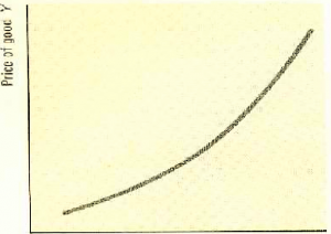
The curve slopes upward, indicating that as the price of a substitute falls, the demand for the good falls. Example of substitute goods includes; butter and margarine, public transport and private cars.
If a fall in the price one good raises the demand for another good, the two goods are said to be complements. In this case, when the price of one good falls, more of that good is consumed and also more of these goods that are complementary to it. This relation will obtain between goods that tend to be consumed together, goods such as motorcars and petrol, bread and butter. This is illustrated in the figure below

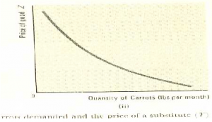
The curve slopes downward, indicating that when the price of a complement falls there is a rise in the quantity demanded.

• Income of the consumer
  Normally we would expect a rise in income to be associated with a rise in the quantity of a good demanded. There are two possible exceptions. In some cases a change in income might leave the quantity demanded completely unaffected. This will be the case with goods for which the desire is completely satisfied after a certain level of income is obtained. Beyond this level, variations in income have no effect on the quantity demanded. This is possible in the case with many of the more inexpensive foodstuffs. It is unlikely for example that the demand for salt would be affected by either an increase in a household income or by a decrease. In the cases of other commodities, it is possible for a rise in income beyond a certain level to lead to a fall in the quantity that the household demands. Such a relation is likely to occur when one commodity is a cheap but inferior substitute for some other commodity. Commodities the demand for which rise as income rise is usually called normal goods. All the three possible relations are illustrated in the figure below.

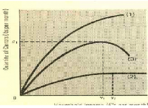
Curve 1 illustrates the case in which a rise in income brings about a rise in purchases at all levels of income. Curve 2 illustrates a case in which purchases rise with income up to a certain point Y2 and then remain unchanged as income varies above that amount. Curve 3 illustrates the case in which purchases first rise with income up a certain level Y1 where purchases are C1, but then fall as income goes beyond that level: the good becomes inferior at incomes higher than Y1.

• Tastes and preference
  If it becomes fashionable amongst middle-class households to have a second car, the flow of expenditure on cars will increase. This does not mean that everybody will buy a second car, but some people will, and quantity demanded will rise. When there is a change in tastes in favour of a commodity, more of the commodity will be demanded even though the price of that commodity, the prices of all other commodities and household income do not change.